The bank computes loans with a finite difference model

Photo credit to Josh Appel

Goals of this article

In the article on continuous solutions to the loan equation, we found that the entire loan could be specified by the loan product, \(rt_\text{term}\), or the initial fraction of payment to interest, \(\phi_0\). In practice, loan payments and interest are not continuous payment rates. If they were, a borrower's bank balance would continuously drop by a few fractions of a cent per second and their balance would change in real-time while they viewed it. Instead, banks charge interest and collect payments at discrete intervals, usually monthly.

In this article, we will show that the mathematical model used in practice to determine a loan balance is the finite difference method for first order ODEs. We will show that both the loan product and number of payment periods during the loan term, \(n\), are necessary to compute all the relevant parameters of the loan. We will find formulas for the principal fraction \(\frac{B_i}{B_0}\), payment to interest \(\phi_i\), and overpay ratio \(\frac{V}{B_0}\) as a function of \(f(rt_\text{term},n)\); the repayment rate \(P\) as a function of \(f(r,t_\text{term},n)\).

Financial interest is calculated as a finite difference solution to a differential equation

Set up the first order differential equation describing a loan using the variable definitions above just as we did in the continuous case here.

Rate of change of loan balance	\( = \)	Interest	\( - \)	Repayment rate
\( \displaystyle \frac{\partial B}{\partial t} \)	\( = \)	\( rB\)	\( - \)	\( P\)

When a bank computes the balance on a loan, they use a recursive function based on the finite difference approximation of this first order ordinary differential equation. This equation can be discretized by approximating \(\partial B = B_{i+1} - B_i\) and \(\partial t = \Delta t\).

$$\begin{align}\frac{B_{i+1} - B_i }{\Delta t} &= B_i r - P\\ B_{i+1} &= B_i r\Delta t - P \Delta t+B_i\end{align}$$

This is the formula commonly programmed into spreadsheet programs to compute loan balances as a function of time:

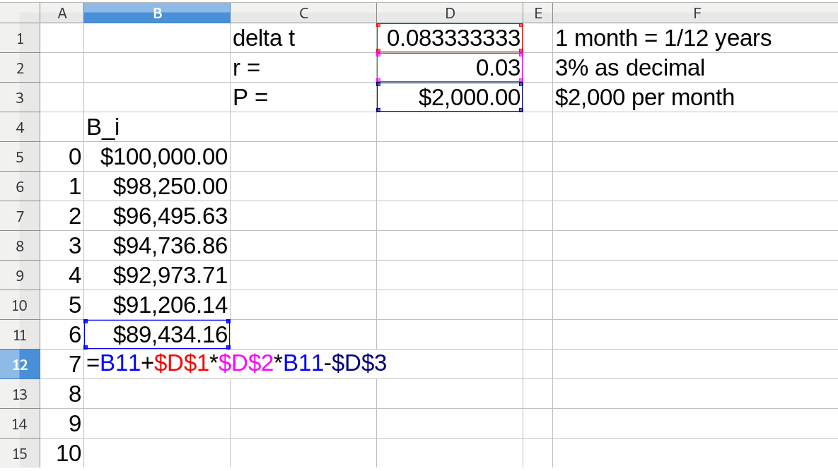
Notice that \(r\Delta t\) is unitless. For example, in this case where \(\Delta t =\) 1 month the conversion appears as follows.

$$r\Delta t = \left[\frac{\%}{\text{year}}\right] \left[\frac{\text{1 year}}{\text{12 month}}\right] \left[\text{1 month}\right] = \frac{r}{12} \; \left[\text{unitless}\right]$$

Solving for useful parameters with an explicit function

Let us expand this recursive function into an explicit one and simplify by defining \(R = 1+r\Delta t \)\(= 1+ \frac{rt_\text{term}}{n}\) for convenience:

$$\begin{align} B_{i+1} &= B_i \left(1+r\Delta t \right) - P\Delta t \\ B_{i+1} &= B_i R- P\Delta t\\ B_{i+1} &= ( B_{i-1}R - P \Delta t )R - P\Delta t \\ B_{i+1} &= \big( ( B_{i-2}R - P\Delta t)R - P\Delta t\big)R - P\Delta t \end{align}$$

Simplify:

$$\begin{align} B_{i+1} &= B_{i}R - P\Delta t \\ B_{i+1} &= B_{i-1}R^2 - P R\Delta t - P\Delta t \\ B_{i+1} &= B_{i-2}R^3 - P R^2\Delta t - PR\Delta t - P\Delta t \end{align}$$

Now we easily see the pattern for a closed-form expression of \(B_i\). Recognize \(\Delta t\) and \(P\) are independent of \(i\) and factor them out of the sum.

$$\begin{align} B_{i} &= B_0R^{i} - P\Delta t \big( R^{i-1} + R^{i-2} + R^{i-3} + \; \dotsc \; + R^{0}\big) \\ B_{i} &= B_0 R^{i} - P\Delta t \sum_{j=1}^{i} R^{j-1} \end{align}$$

From this follows an expression for the payment as a function of the loan term, rate and payment/maturation frequency (set \(B_n = 0\)). The number of payment cycles is a function of the term of the loan \(n=t_\text{term}/\Delta t\).

$$B_0 R^{t_\text{term}/\Delta t} = P \Delta t \sum_{i=0}^{t_\text{term}/\Delta t-1} R^{i} $$ $$\frac{P}{B_0} = \frac{ (1+r\Delta t)^{t_\text{term}/\Delta t}}{\Delta t \sum^{(t_\text{term} /\Delta t)-1}_{i=0} (1+r\Delta t)^i } = \frac{ n R^{n}}{t_\text{term} \sum^{n-1}_{i=0} R^i } $$

From here we can derive an equation for \(\frac{B_i}{B_0}\) that is solely a function of the total number of payment periods, \(n\), and the loan product, \(rt_\text{term}\).

$$\frac{B_{i}}{B_0} = R^{i} - \frac{ R^{n}}{ \sum^{n-1}_{k=0} R^k } \sum_{j=1}^{i} R^{j-1} \quad \text{where} \quad R = 1+ \frac{rt_\text{term}}{n}$$

The overpay ratio follows easily. \(V\) is the total amount repaid and \(V= Pt_\text{term}\). The ratio between what is repaid and what is borrowed is \(\frac{V}{B_0}\). This can be viewed as a function of \((r, \, t_\text{term}, \, \Delta t)\) or as a function of \((rt_\text{term}, \, n)\).

$$\begin{align} \frac{V}{B_0} &= \frac{P }{B_0}t_\text{term} \\ \frac{V}{B_0} &= \frac{ t_\text{term} (1+r\Delta t)^{t_\text{term}/\Delta t}}{\Delta t \sum^{(t_\text{term} /\Delta t)-1}_{i=0} (1+r\Delta t)^i}\\ \frac{V}{B_0} &= \frac{ n (1+\frac{rt_\text{term}}{n})^{n} }{\sum^{n-1}_{i=0} (1+\frac{rt_\text{term}}{n})^i } \end{align}$$

We can also derive an expression for the fraction of each payment put to interest as a function of \(i\), \(rt_\text{term}\), and \(n\).

$$\begin{align} \phi_i &= \frac{rB_{i}}{P} = \frac{rB_0}{P} R^{i} - r\Delta t \sum_{j=1}^{i} R^{j-1}\\ \phi_i &= \phi_0 R^{i} - \frac{rt_\text{term}}{n} \sum_{j=1}^{i} R^{j-1} \\ \phi_i &= \frac{rt_\text{term}}{n}\left( \frac{\sum_{j=1}^{n} R^{j-1}}{ R^n} R^{i} - \sum_{j=1}^{i} R^{j-1} \right) \quad \text{where} \quad R = 1+ \frac{rt_\text{term}}{n} \end{align}$$

When we plot \(\phi_i\) vs \(\tau\) with increasing \(n\), we eventually approximate the continuous solution (recall that \(\tau=i/n\)). The continuous solution becomes recognizable by \(n= \) 20 and becomes visually indistinguishable around \(n= \) 200. A future article will discuss the error between the continuous and discrete solutions when solving for the overpay ratio or the repayment rate.