
Photo credit to Colin Behrens
This is a (lightly edited) conference paper I published in 2022 at the Digital Pipelines Solution Forum [1]. It describes the first commercially useful neural network I produced. If you were to drop a magnetometer down a steel pipeline and measure the magnetic flux at 200 hz, this neural network would be able to interpret that data and produce a list of joint locations in time. Obviously this problem has a narrow application. We might be the only company in the world that could benefit from solving this particular problem but for us it is incredibly valuable. Prior to the development of this algorithm, the company paid data analysts like me to manually identify joint locations in a GUI by clicking on them one at a time. In a line with 3,000 joints, this might take two to four days. Running on a modern laptop, my neural network produces a result with false positive and false negative rates below 5% in under three minutes. Manually reviewing the joint list with these error rates is between three and ten times faster than manual identification from scratch.
As we collect more training data, we expect false positive and false negative rates to drop below 1%. For context, the discrepancy between two different manual labelers is around 0.5-2%. We expect to beat human level performance in the next two to five years.
In 2016, pipeline failures in the North America resulted in the uncontrolled release of 2,000 metric tons of hydrocarbons (both liquid and gas) [2]. Pigs a vital part of pipeline maintenance. The term pig refers to any device placed inside a pipeline, pushed through from entrance to exit usually with fluid pressure. There are many varieties of pig; some are made of steel and scrape along the wall removing deposits; some are foam and do the same thing but less aggressively and with the ability to traverse tighter bends and diameter changes; some are equiped with tracking devices making them easier to locate if stuck in the pipe; some are filled with sensors designed to detected leaks or corrosion. The primary tools of pipeline integrity management since the 1980s are magnetic flux leakage (MFL) and ultra sound devices. These are "smart pigs." However, the problem of unpiggable pipelines, due to tight bends, non-circular valves, diameter changes or unknown geometry continues to cause problems in the pipeline inspection industry [2,3]. Approximately 70% of US gas lines were built before modern inline inspection (ILI) was a viable technology [4]. As of 2012, industry surveys indicate ~40% of gas pipelines in North America are unpiggable [5]. More recent technologies to address unpiggable lines began in the early 2000s [6,7].
Regardless of the technology, determining location within the pipe has always been a challenge. Traditional ILI tools use odometer wheels but slippage remains a problem, particularly in lines with heavy deposits or rough surfaces [8]. Inaccuracies in distance can be minimized by using external above ground markers (AGMs). AGMs come in magnetic, acoustic, or geophone array varieties [9,10,11]. However, AGM systems are expensive, often cannot be used in crowded urban areas, and are limited in accuracy depending on the depth of the pipeline. Multisensor free-floating devices solve the localization problem with an alternative method which has its own set of challenges and strengths. Welds identified from the magnetometer data are a primary component of the conversion from measurement time to measurement distance [12]. The neural network (NN) we are presenting here successfully automates the detection of pipe welds in steel pipes from residual magnetometer data with near human level performance. Automation of this critical bottleneck dramatically improves the scalability of multisensor free-floating devices.
Joints morphology, as detected by residual magnetometry, is highly heterogenous. Some pipeline joints can be found with a simple peak search. Others show up as subtle increases in oscillation frequency. Some are so subtle that they can only be determined by considering the average joint spacing in the surrounding area. Because joint identification lacks precise articulable attributes which might lend it to imperative programming [12,13], a NN is the most promising solution.

[Caption] Examples of the diversity of joint morphology in residual magnetometry measurements in steel pipelines. Upper and lower plots show data from different sections of the same survey with the same x and y scale. In the upper graph, the joints could be choosen with an off-the-shelf peak finding algorithm. In the lower graph, joints were manually identified by looking for small areas of increased signal frequency and interpolating between areas of high confidence to positively identify joints in areas of low confidence.
The most successful deep learning strategies were developed in the context of computer vision (aka image processing). Let's define some terms. Classification is any algorithm that takes a large input and returns a class label from a predetermined set. Pixel values as input and "is this a dog or cat?" as an output is a classification problem. It is critically important that we know in advance that the photo will be a cat or dog. This applies equally well to any number of predefined categories. It need not be binary. Segmentation is the same concept but applied to each data point. This is the "highlight all the pixels of a cat in this image" type of problem.
To develop an automated joint detection system we conceptuallize this as a 1D segmentation problem. We apply a label to each data point (joint or no-joint), and design a NN to classify each point. The network takes the four magnetic vectors as inputs (\(m_x\), \(m_y\), \(m_z\), and \(m_t\) where \(m_t = (m_x^2 + m_y^2 + m_z^2)^{0.5})\) and returns two (\(y_1\), \(y_2\)). The joint likelihood vs position function is given by a softmax \(p = \frac{e^{y_2}}{e^{y_1} + e^{y_2}}\). See figure below.
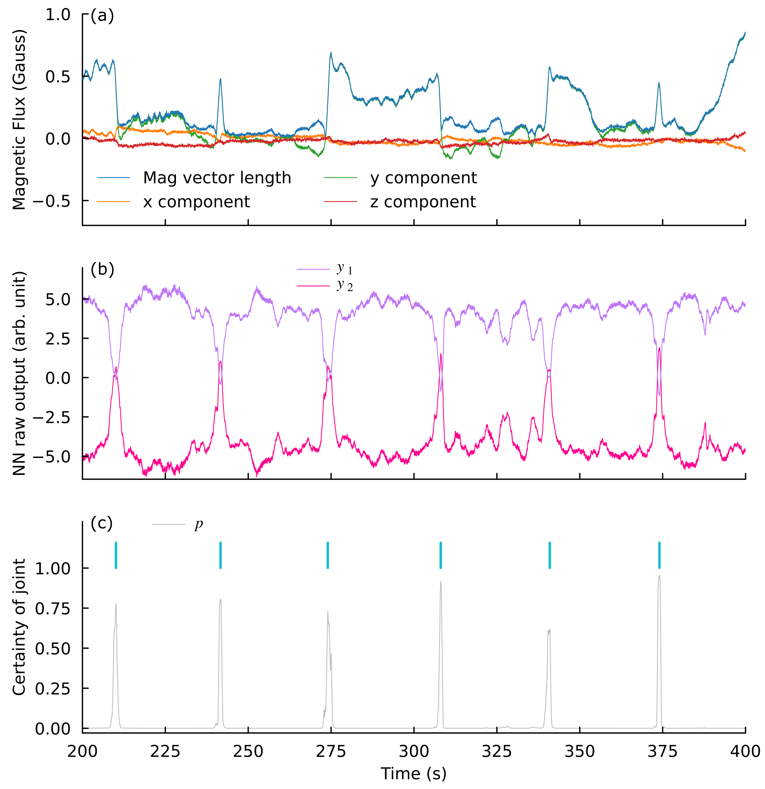
[Caption] (a) Inputs to NN. Because no natural normalization basis is present and because the values are on the order of 1, no normalization was applied to the input data. (b) Raw output of the NN in arbitrary units. (c) Softmax of NN output vectors from (b) gives a "certainty of joint" measurement. Peak search on this array gives a joint list (cyan).
Since the publication of the original paper on UNet in 2015 [14], fully convolutional NN have become the gold standard for segmentation problems. There are now thousands of published variations and application of UNet. The original paper has 39,554 citations as of 2022-03-23. Our application of UNet requires several modifications. First, because we have 1D data instead of 2D data, our data points are further apart and the receptive fields must be increased to accomodate this increased distance. Second, the precision of the segmentation in joint identification is less precise than in medical image segmentation. Therefore we do not need the output arrays to be as large as the input arrays. Third, because our data is pipeline magnetics and not micrographs of cells, the data augmentations appropriate for training are not the same.
Broadening the receptive field to include at least several joints provides the NN with the context that manual joint identification utilizes. What is likely a joint in the context of one pipeline's magnetic signature may be part of the normal fluctuations within a pipe segment on another line. When manually identifying joints, we look for repeated signatures with approximately equal spacing. For the NN to mimic this process, the receptive field of the deepest neurons must include multiple joints. This insight is the most critical part of the adaptation of UNet to 1D segmentation.
The 572x572 square pixel images of the original UNet have 327,184 data points per image but no data point is more than 571 steps away from any other data point. With a magnetometer sampling frequency of 200 Hz and 250 second snapshots, our input data is 51,840 data points long. However, the maximum distance between data points in 51,839 rather than 571. By shifting from 2D to 1D, we can reduce our input by 85% and yet the maximum distance between points can increase by 90x. As information travels down the encoder side of the UNet, we need a broader receptive field to capture context from a wider area to make accurate classifications of each point.
The receptive field of a neuron in a NN of convolutional and pooling layers [15] is given by
where \(k_l\) is the kernel at layer \(l\) and \(s_i\) is the stride of layer \(i\). For the original UNet, the receptive field of the first 14 layers which make up encoder is 140x140 pixels. By increasing the stride of the first of each pair of convolutions to 2 and increase the kernel and stride of the the max pooling layers to 3, we can increase the receptive field from 140 to 10,367. This increase is what allows the encoder to place the magnetometer data in appropriate context within the rest of the line.
We used transpose convolutions to reverse the compressions of the max pool and convolutional layers with stride 2. By selecting an input array length evenly divisible by the strides of all the encoder layers, we were able to design a network which required no cropping before appending encoder layers into the decoder side of the network. This produced a slight increase in training performance and adds a cleanliness to the network design.
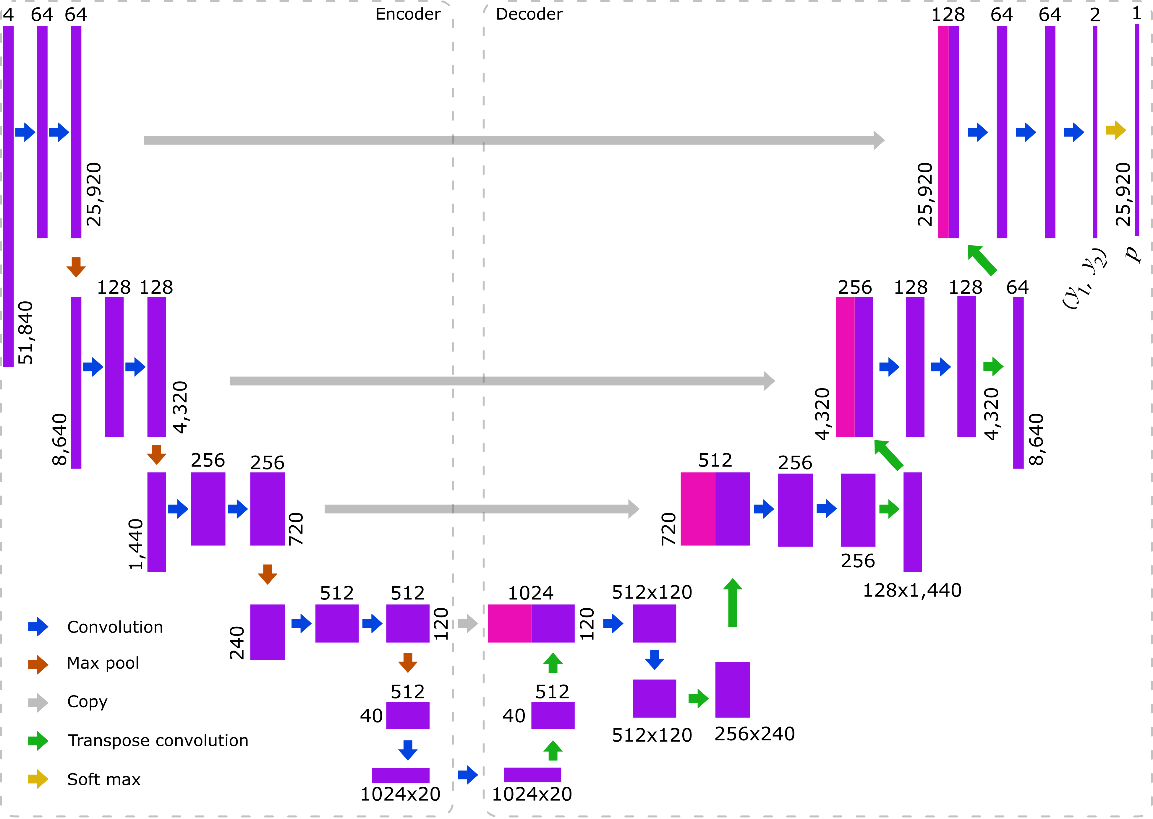
[Caption] Architecture of fully convolutional UNet for 1D segmentation. Rectangular dimensions are not proportional to length because the length of the tensors changes by a factor of 2,600 as it moves through the network. All convolutional layers have a kernel of 3. On the encoder side of the network, the stride is 2 or 1 for the first or second in each pair, respectively. On the decoder side, the stride is 1 for all convolutional layers. All transpose convolutional layers have a kernel of 3; the stride is 2 or 3 for the first or second in each pair respectively. Max pool layers have a kernel and stride of 3. ReLU activations functions follow each convolutional or transpose convolutional layer.
Despite much attention, the question of how much data a NN requires for training remains an active research area [16,17]. Most estimates are between 10 and 1000 times the number of parameters in the model. However, we have a NN with 12.6 million parameters and only ~100,000 examples of joints. Those are not even independent training samples because the NN needs multiple joints per sample to train. However, we are fortunate in several ways. First we have a large number of data augmentations available which allowed us to create 3 million training samples. Second, even with the augmentations, this NN converged and generalized with two orders of magnitude less training data than would typically be expected for a NN this size. Therefore, we expect the network to improve as more data is incorporated into the training library.
To generate an augmented data sample
- Select random survey
- Select random subset of survey 37.5k to 70k data points long
- Resample by linear interpolation to 50k data points (stretch or compress in x)
- Multiply each component by random scaler value from 0.7 to 1.33 (stretch or compress in y)
- With 50% probability, reverse the sample (mirror in x)
- Randomly reorder x, y, z components. Because measurements are taken free floating, the orientation of the sensor is random so random reordering of components is a valid augmentation strategy.
By using these augmentations, we were able to train a NN of 12.7 million parameters using only 111 surveys containing 90,898 examples of joints.
The training data y values are defined as a discrete list of points but our output is a segmentation output. To make a ground truth tensor suitable for a segmentation algorithm, we define the ground truth as "joint" within a window of 50 data points and "not joint" everywhere else. This first approximation performed near human accuracy without attempting to correct for joint width variability in our training data.
This network was trained using a standard cross-entropy loss function without applying different weights to different data points. The original UNet was interested in the edges of cells. Weighting the loss function higher at the boundaries forced the network to precisely localize predictions. In this application, we have the opposite situation. It is most important to learn the classes of the data points in the center of the joint region but not at all important to learn the exact edges of the target segmentation. If anything, the fuzzy borders of the target segmentation lends itself to a loss weighting scheme inverted from the original UNet. Implementation of such a weight scheme was not required for the results presented here. However, it is possible that analogous problems may benefit from such training weights, either to reduce the training time or to improve the training robustness.
This NN trained for 100,000 cycles with a learning rate of 0.1 and minibatches of 30 samples. At the end of that time, it performed joint identification on a validation survey with 2,981 joints. It correctly identified 2,839 with 142 false negatives and 33 false positives, 4.8% and 1.1% respectively. Human level performance (as measured by agreement between independent manual labelers) has false positive and false negative rates of approximately 0.1 to 2% depending on the pipeline. Our NN is performing slightly below human level accuracy.
Because the network was trained with surprisingly little data, we will likely see significant improvements as our training data library grows. There is also a specific use case where acceleration and gyroscopic data are informative. Some surveys are performed with the sensor device attached to a cleaning pig. As the pig hits welds, the acceleration and gyroscope sensors register the impact. Depending on how tight the pig fits in the pipe and how much the weld seam protrudes, the size of this signal can vary from non-existent to completely unambiguous. A similar NN which incorporates acceleration, gyroscopic, and magnetic measurements will likely perform better on cleaning pig surveys.
[1] "Neural networks for pipeline joint detection," Digital Pipeline Solutions Forum, 2022.
[2] "A review on pipeline integrity management utilizing in-line inspection data," Engineering Failure Analysis, vol. 92, pp. 222—239, 2018.
[3] "An overview of major methods for inspecting and monitoring external corrosion of on-shore transportation pipelines," Corrosion Engineering, Science and Technology, vol. 50, pp. 226—235, 2015.
[4] "Report to the National Transportation Safety Board on Historical and Future Development of Advanced In-Line Inspection Platforms for Use in Gas Transmission Pipelines," 2012.
[5] "Ultimate Guide to Unpiggable Pipelines," 2013.
[6] "SmartBall: a new approach in pipeline leak detection," International Pipeline Conference, vol. 48586, pp. 117—133, 2008.
[7] "Leak detection and prevention using free-floating in-line sensors," Pipeline Pigging and Integrity Management, 2019.
[8] "Review of sensor technologies for in-line inspection of natural gas pipelines," Sandia National Laboratories, 2002.
[9] "Research on Above Ground Marker System of pipeline Internal Inspection Instrument Based on geophone array," 2010 6th International Conference On Wireless Communications Networking and Mobile Computing, pp. 1—4, 2010.
[10] "A novel algorithm for acoustic above ground marking based on function fitting," Measurement, vol. 46, pp. 2341—2347, 2013.
[11] "Establishment of theoretical model of magnetic dipole for ground marking system," 2017 29th Chinese Control And Decision Conference (CCDC), pp. 6134—6138, 2017.
[12] "Defect localization using free-floating unconventional ILI tools without AGMs," Pipeline Pigging and Integrity Management, 2022.
[13] "Pipers; an inline screening tool for unpiggable pipelines," Unpiggable Pipeline Solutions Forum, 2019.
[14] "U-Net: Convolutional Networks for Biomedical Image Segmentation," Medical Image Computing and Computer-Assisted Intervention (MICCAI), vol. 9351, pp. 234—241, 2015.
[15] "Computing receptive fields of convolutional neural networks," Distill, vol. 4, pp. e21, 2019.
[16] "Is your dataset big enough? Sample size requirements when using artificial neural networks for discrete choice analysis," Journal of Choice Modelling, vol. 28, pp. 167—182, 2018.
[17] "Estimating the required training dataset size for transmitter classification using deep learning," 2019 IEEE International Symposium On Dynamic Spectrum Access Networks, pp. 1—10, 2019.